Tutorial 6: EPR without HFSS — Purely Numerical Workflow

pyEPR’s numerical diagonalization does not require Ansys HFSS. If you already know (or can compute from another source) the three ingredients:

Quantity	Symbol	Units	How to get it
Linearised mode frequencies	freqs	GHz	EM solver, circuit model, or experiment
Junction inductances at the bias point	Ljs	H	Circuit design / fabrication
Reduced zero-point flux fluctuations	phi_zpf	dimensionless	From EPR integrals or black-box quantisation

you can call epr_numerical_diagonalization directly and obtain dressed frequencies and the full dispersive-shift / anharmonicity matrix — no HFSS licence, no Ansys installation, no COM calls.

This tutorial demonstrates the workflow for four common circuit types:

1. Single transmon — textbook single-junction qubit

2. Transmon + readout resonator — two-mode coupled system

3. Fluxonium — strongly anharmonic, requires use_full_cos=True

4. Custom potential — user-supplied V(φ) via make_nonlinear_potential

References

• Z. K. Minev et al., Energy-participation quantization of Josephson circuits, npj Quantum Information 7, 131 (2021) (arXiv:2010.00620) — introduces pyEPR and the EPR framework.

• S. E. Nigg et al., Black-box superconducting circuit quantization, Phys. Rev. Lett. 108, 240502 (2012) — black-box quantisation (BBQ) that black_box_hamiltonian implements.

• J. Koch et al., Charge-insensitive qubit design derived from the Cooper pair box, Phys. Rev. A 76, 042319 (2007) — transmon.

• V. E. Manucharyan et al., Fluxonium: Single Cooper-pair circuit free of charge offsets, Science 326, 113 (2009) — fluxonium.

• A. Petrescu, C. T. Hann, Z. K. Minev et al., arXiv:2411.15039 — full-cosine EPR for very anharmonic circuits.

Series navigation: ← Tutorial 5: Generic Junction Potential & Fluxonium

import numpy as np
import matplotlib.pyplot as plt

from pyEPR.calcs.back_box_numeric import (
    epr_numerical_diagonalization,
    make_nonlinear_potential,
)
from pyEPR.calcs.constants import hbar, fluxQ

# Useful physical constants
Phi0_over_2pi = fluxQ   # Φ₀/2π in Wb  (the reduced flux quantum)
print(f"Φ₀/2π = {fluxQ:.4e} Wb")

Φ₀/2π = 3.2911e-16 Wb

---

Background: what are freqs, Ljs, phi_zpf?

Linearised mode frequencies freqs

The EPR framework replaces each Josephson junction by its linearised inductance \(L_j = (\Phi_0/2\pi)^2 / E_J\) and finds the normal modes of the resulting linear circuit. These are the frequencies that an EM solver (HFSS) or a lumped-circuit model would give for the system with the junctions replaced by inductors.

For a transmon with \(E_J/h = 20\,\text{GHz}\) and \(E_C/h = 0.3\,\text{GHz}\), the plasma frequency is \(\omega_p/2\pi = \sqrt{8 E_J E_C}/h \approx 6.9\,\text{GHz}\).

Junction inductance Ljs

\(L_j = (\Phi_0/2\pi)^2 / E_J\). For \(E_J/h = 20\,\text{GHz}\): $\(L_j = \frac{(\Phi_0/2\pi)^2}{h \times 20\,\text{GHz}} \approx 8.3\,\text{nH}\)$

Zero-point flux fluctuation phi_zpf

The reduced ZPF of mode \(m\) across junction \(j\) is $\(\varphi_{\rm zpf}^{(m,j)} = \sqrt{\frac{\hbar \omega_m}{2} \cdot \frac{L_j}{(\Phi_0/2\pi)^2}} = \sqrt{\frac{E_m}{2 E_J}}\)$

where \(E_m = \hbar\omega_m\) is the zero-point energy of the mode. For a single-mode transmon this is just \(\phi_{\rm zpf} = (2 E_C/E_J)^{1/4}\) (the standard result).

The phi_zpf array has shape (n_modes × n_junctions).

---

1 — Single transmon

Setting up parameters from \(E_J\) and \(E_C\)

A transmon has \(E_J \gg E_C\). The plasma (linearised) frequency is \(\omega_p/2\pi = \sqrt{8 E_J E_C}/h\), and the single-mode ZPF is \((2 E_C / E_J)^{1/4}\).

h = 6.626e-34   # Planck constant

# Transmon energies (in GHz × h, converted to Joules)
EJ_GHz = 20.0   # Josephson energy
EC_GHz =  0.3   # charging energy

EJ = EJ_GHz * 1e9 * h   # Joules
EC = EC_GHz * 1e9 * h

# Linearised plasma frequency (GHz)
f_plasma = np.sqrt(8 * EJ * EC) / h / 1e9
print(f"Plasma frequency:  {f_plasma:.3f} GHz")

# Josephson inductance (H)
Lj = fluxQ**2 / EJ
print(f"Josephson inductance: {Lj*1e9:.2f} nH")

# Zero-point phase fluctuation (dimensionless)
phi_zpf_transmon = (2 * EC / EJ) ** 0.25
print(f"phi_zpf:  {phi_zpf_transmon:.4f}  (≪ 1, weakly anharmonic — truncated series works)")

Plasma frequency:  6.928 GHz
Josephson inductance: 8.17 nH
phi_zpf:  0.4162  (≪ 1, weakly anharmonic — truncated series works)

# Pack into arrays: shape = (n_modes,) and (n_modes × n_junctions)
freqs   = np.array([f_plasma])            # 1 mode, GHz
Ljs     = np.array([Lj])                  # 1 junction, H
phi_zpf = np.array([[phi_zpf_transmon]])  # shape (1 mode, 1 junction)

f_ND, chi_ND = epr_numerical_diagonalization(
    freqs, Ljs, phi_zpf, cos_trunc=8, fock_trunc=15
)

print(f"Dressed frequency:    {np.real(f_ND[0])/1e9:.4f} GHz")
print(f"Anharmonicity (χ/2π): {np.real(chi_ND[0,0]):.1f} MHz")

# Compare with analytic result: α ≈ -EC (in the transmon limit)
print(f"\nAnalytic anharmonicity ≈ EC/h = {EC_GHz*1e3:.0f} MHz  (pyEPR: {np.real(chi_ND[0,0]):.0f} MHz)")

INFO 04:24AM [make_dispersive]: Starting diagonalization (15×15 matrix)

INFO 04:24AM [make_dispersive]: Diagonalization complete

Dressed frequency:    6.6135 GHz
Anharmonicity (χ/2π): 336.9 MHz

Analytic anharmonicity ≈ EC/h = 300 MHz  (pyEPR: 337 MHz)

---

2 — Transmon coupled to a readout resonator

A two-mode system: the transmon mode (qubit) and a readout cavity. In this model the junction participates in both modes via the participation ratios \(\varphi_{\rm zpf}\).

• freqs[0] = qubit linearised frequency

• freqs[1] = readout resonator frequency

• phi_zpf[0, 0] = qubit ZPF across the junction (large)

• phi_zpf[1, 0] = readout ZPF across the junction (small — dispersive coupling)

The off-diagonal chi_ND[0,1] gives the dispersive shift \(\chi_{qr}\).

freqs_2mode   = np.array([5.5, 7.0])           # qubit, resonator (GHz)
Ljs_2mode     = np.array([Lj])                  # single junction (H)

# phi_zpf: shape (n_modes=2, n_junctions=1)
# Qubit mode has large ZPF; resonator mode has small ZPF across the junction
phi_zpf_2mode = np.array([[0.20],   # qubit participation
                           [0.02]])  # resonator participation

f2, chi2 = epr_numerical_diagonalization(
    freqs_2mode, Ljs_2mode, phi_zpf_2mode,
    cos_trunc=8, fock_trunc=10,
)

print("Dressed frequencies:")
print(f"  Qubit:    {np.real(f2[0])/1e9:.4f} GHz")
print(f"  Readout:  {np.real(f2[1])/1e9:.4f} GHz")
print()
print("χ matrix (MHz):")
chi2_r = np.real(chi2)
print(f"  χ_qq (qubit anharmonicity): {chi2_r[0,0]:.2f} MHz")
print(f"  χ_rr (readout self-Kerr):   {chi2_r[1,1]:.3f} MHz")
print(f"  χ_qr (dispersive shift):    {chi2_r[0,1]:.3f} MHz")

INFO 04:24AM [make_dispersive]: Starting diagonalization (100×100 matrix)

INFO 04:24AM [make_dispersive]: Diagonalization complete

Dressed frequencies:
  Qubit:    5.4839 GHz
  Readout:  6.9998 GHz

χ matrix (MHz):
  χ_qq (qubit anharmonicity): 15.89 MHz
  χ_rr (readout self-Kerr):   0.002 MHz
  χ_qr (dispersive shift):    0.308 MHz

---

3 — Fluxonium: exact cosine is essential

For a fluxonium-type circuit the zero-point phase fluctuation is large (\(\varphi_{\rm zpf} \sim 1{-}3\)). The truncated Taylor series of \(\cos\varphi - 1 + \varphi^2/2\) diverges in this regime; set use_full_cos=True to use the matrix-exponential path instead.

See arXiv:2411.15039 for a detailed comparison.

# Fluxonium parameters: large inductance → large phi_zpf
freqs_fl   = np.array([0.5])     # GHz  (plasmon mode, ~0.5–2 GHz typical)
Ljs_fl     = np.array([500e-9])  # H    (large superinductance Lj ≫ standard)
phi_zpf_fl = np.array([[2.0]])   # dimensionless (large!)

print("Fluxonium — comparing truncation levels:")
print()

results = {}
for trunc, label in [(4, 'cos_trunc=4'), (8, 'cos_trunc=8'), (16, 'cos_trunc=16')]:
    f, chi = epr_numerical_diagonalization(
        freqs_fl, Ljs_fl, phi_zpf_fl,
        cos_trunc=trunc, fock_trunc=25
    )
    results[label] = (np.real(f[0]), np.real(chi[0,0]))
    print(f"  {label:15s}:  f = {np.real(f[0])/1e9:.4f} GHz,  χ = {np.real(chi[0,0]):.2f} MHz")

f_exact, chi_exact = epr_numerical_diagonalization(
    freqs_fl, Ljs_fl, phi_zpf_fl,
    fock_trunc=25, use_full_cos=True    # ← recommended for fluxonium
)
print(f"  {'use_full_cos':15s}:  f = {np.real(f_exact[0])/1e9:.4f} GHz,  χ = {np.real(chi_exact[0,0]):.2f} MHz  ← exact")

print()
for label, (f_val, chi_val) in results.items():
    err = abs(f_val - np.real(f_exact[0])) / abs(np.real(f_exact[0]))
    print(f"  {label}: relative error vs. exact = {err:.1%}")

INFO 04:24AM [make_dispersive]: Starting diagonalization (25×25 matrix)

INFO 04:24AM [make_dispersive]: Diagonalization complete

INFO 04:24AM [make_dispersive]: Starting diagonalization (25×25 matrix)

INFO 04:24AM [make_dispersive]: Diagonalization complete

INFO 04:24AM [make_dispersive]: Starting diagonalization (25×25 matrix)

INFO 04:24AM [make_dispersive]: Diagonalization complete

INFO 04:24AM [make_dispersive]: Starting diagonalization (25×25 matrix)

INFO 04:24AM [make_dispersive]: Diagonalization complete

Fluxonium — comparing truncation levels:

  cos_trunc=4    :  f = 57729.3828 GHz,  χ = 57729380.03 MHz
  cos_trunc=8    :  f = 602249.4553 GHz,  χ = 602251647.74 MHz
  cos_trunc=16   :  f = 1474.8288 GHz,  χ = 1476793.06 MHz
  use_full_cos   :  f = 39.0206 GHz,  χ = 40984.63 MHz  ← exact

  cos_trunc=4: relative error vs. exact = 147846.0%
  cos_trunc=8: relative error vs. exact = 1543315.2%
  cos_trunc=16: relative error vs. exact = 3679.6%

Fock-space convergence check

Always verify that the result is converged with respect to fock_trunc.

fock_range = [10, 15, 20, 25, 30]
f_vals  = []
chi_vals = []

for ft in fock_range:
    f, chi = epr_numerical_diagonalization(
        freqs_fl, Ljs_fl, phi_zpf_fl,
        fock_trunc=ft, use_full_cos=True
    )
    f_vals.append(np.real(f[0])/1e9)
    chi_vals.append(np.real(chi[0, 0]))

fig, axes = plt.subplots(1, 2, figsize=(10, 3.5))
axes[0].plot(fock_range, f_vals, 'o-', lw=2)
axes[0].set(xlabel='Fock truncation', ylabel='Dressed frequency (GHz)',
            title='Frequency convergence (fluxonium)')
axes[1].plot(fock_range, chi_vals, 'o-', lw=2, color='C1')
axes[1].set(xlabel='Fock truncation', ylabel='χ (MHz)',
            title='Anharmonicity convergence (fluxonium)')
for ax in axes:
    ax.grid(True, alpha=0.3)
plt.tight_layout()
plt.show()

print(f"Converged values:  f = {f_vals[-1]:.4f} GHz,  χ = {chi_vals[-1]:.2f} MHz")

INFO 04:24AM [make_dispersive]: Starting diagonalization (10×10 matrix)

INFO 04:24AM [make_dispersive]: Diagonalization complete

INFO 04:24AM [make_dispersive]: Starting diagonalization (15×15 matrix)

INFO 04:24AM [make_dispersive]: Diagonalization complete

INFO 04:24AM [make_dispersive]: Starting diagonalization (20×20 matrix)

INFO 04:24AM [make_dispersive]: Diagonalization complete

INFO 04:24AM [make_dispersive]: Starting diagonalization (25×25 matrix)

INFO 04:24AM [make_dispersive]: Diagonalization complete

INFO 04:24AM [make_dispersive]: Starting diagonalization (30×30 matrix)

INFO 04:24AM [make_dispersive]: Diagonalization complete

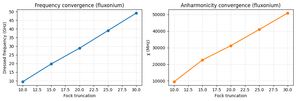
Converged values:  f = 49.1677 GHz,  χ = 50884.35 MHz

---

4 — Custom potential via make_nonlinear_potential

If the junction element has a potential that is not a simple cosine — for example an asymmetric SQUID, a flux-biased junction, or a non-standard Josephson element — you can provide an arbitrary scalar function and let pyEPR construct the nonlinear correction automatically.

See Tutorial 5 for a detailed treatment. Here we show the minimal usage pattern.

# Asymmetric SQUID: effective potential for the common-mode phase
#   V(φ) = cos(φ)·cos(φ_ext) + d·sin(φ)·sin(φ_ext)
# where d = (Ej1 - Ej2)/(Ej1 + Ej2), φ_ext = external flux (reduced)

phi_ext = 0.3   # rad
d       = 0.1   # junction asymmetry

def V_squid(phi):
    return np.cos(phi) * np.cos(phi_ext) + d * np.sin(phi) * np.sin(phi_ext)

phi_min_squid = np.arctan(-d * np.tan(phi_ext)) % np.pi
print(f"Potential minimum at phi_min = {phi_min_squid:.4f} rad")

nl_squid = make_nonlinear_potential(V_squid, phi_min=phi_min_squid)

f_sq, chi_sq = epr_numerical_diagonalization(
    freqs, Ljs, phi_zpf,        # reuse single-transmon params from §1
    fock_trunc=15,
    non_linear_potential=nl_squid,
)

print(f"Asymmetric SQUID:  f = {np.real(f_sq[0])/1e9:.4f} GHz,  χ = {np.real(chi_sq[0,0]):.2f} MHz")

INFO 04:24AM [make_dispersive]: Starting diagonalization (15×15 matrix)

INFO 04:24AM [make_dispersive]: Diagonalization complete

Potential minimum at phi_min = 3.1107 rad
Asymmetric SQUID:  f = 7.2082 GHz,  χ = -234.67 MHz

---

Interpreting the output

Output	Meaning
f_ND[m]	Dressed frequency of mode m in GHz. Shift from linearised frequency reflects the Lamb shift from the junction nonlinearity.
chi_ND[m, m]	Self-anharmonicity of mode m in MHz. For a qubit, this is the anharmonicity α = ω₁₂ − ω₀₁. Positive = red-shifted (normal sign convention).
chi_ND[m, n] (m≠n)	Dispersive coupling between modes m and n in MHz.

Tips for reliable results

1. Fock truncation: always check convergence by running at two fock_trunc values. A rule of thumb: fock_trunc ≥ 10 / phi_zpf per junction.

2. Cosine truncation: for phi_zpf ≲ 0.3 the default cos_trunc=8 is accurate to < 0.1 %. For phi_zpf ≳ 1, always use use_full_cos=True.

3. Units: freqs must be in GHz, Ljs in Henries. The function asserts this and rejects values that look like they might be in the wrong units.

4. Multi-junction: phi_zpf is shape (n_modes, n_junctions) — each column is one junction, each row is one mode.

Obtaining phi_zpf without HFSS

If you are using a lumped-circuit model, the ZPF can be derived analytically from the energy participation of each mode in each junction inductance:

\[\varphi_{\rm zpf}^{(m,j)} = \sqrt{\frac{\hbar\omega_m}{2} \cdot \frac{L_j}{(\Phi_0/2\pi)^2}} = \sqrt{\frac{p_{mj}}{2} \cdot \frac{\hbar\omega_m}{E_{J,j}}}\]

where \(p_{mj}\) is the energy participation ratio of mode m in junction j. For a simple transmon with a single LC mode: \(p_{11} = 1\) and \(\varphi_{\rm zpf} = (2E_C/E_J)^{1/4}\) (the textbook result).